Modelling nature: A physicist′s viewpoint

INTRODUCTION

Nowadays, physics is often seen as the science of the inanimate world, from the very small (particle physics, quantum mechanics), to the very large (astronomy and cosmology), but this is only a recent restriction. Etymologically, physics comes from the Greek verb which means I appear and grow spontaneously like a cell or a plant. From this verb comes the substantive , which means nature and the related adjective . Hence, physics, or is the science of nature, and its object is the totality of the real world. Beyond, begins the realm of metaphysics.

It is the reductionist approach which first permitted some fields of science to obtain results such as laws and equations: astronomy became a predictive science when planets were ‘reduced’ to points in the equations of Kepler and Newton. Because the sciences dealing with life could not for a long time benefit from this kind of approach, they were left out of mainstream physics. But recent progress in three very different directions – firstly, measuring methods and data analysis, secondly, theoretical tools, and lastly, computers – have drastically changed the picture, and now life sciences can be addressed by the tools of physics.

Experimental physics has given a large number of new tools to study nature of which the most notable are microscopy, ¹⁴C radiometric dating, satellite imagery, and DNA analysis. Simultaneously, statistics and data analysis methods have been developed making these measurements exploitable. Life sciences have thus become quantitative sciences.

On the theoretical side, Friedrich Hayek, (1899–1992, Nobel prize in economics in 1974), was one of the first to introduce the concept of complexity in science, and he distinguished the possibility of predicting the behaviour of a simple system by using a law (an equation relating a small number of variables), from the possibility of predicting the behaviour of a complex system by using a model, and this applied to such fields as economy, biology, ecology, and psychology. Note that although there is no strict definition of a complex system, there is some consensus that it should: (a) have many components (b) have a behaviour which is not trivial to predict (c) exhibit some kind of emerging properties such as self-organization. Because of the large (and often huge) number of actors and relations in such systems, it is impossible to find simple laws describing their behaviour, and a very large number of equations and variables are necessary, thus constituting a model. This large number of equations cannot be solved by hand, and this is where the third element is crucial: the appearance of computers renders feasible the study of the evolution of the sets of equations which constitute the models. Modelling complex systems such as those encountered in meteorology, climatology, economy, social sciences, neurosciences, organic chemistry, molecular biology, psychology, and ecology is now possible using the methods of physics and supercomputers.

Surprisingly (but is it really a coincidence?), it is at this same present time that direct human influence on our planet is becoming worrying. Short term problems have to be addressed urgently if we want to maintain the Earth as viable for mankind. And for this, it is no longer enough to discover, describe, and classify new species; one needs a real understanding of climate change, of ecosystems dynamics, of emerging diseases, and so on, in order to predict the impacts of human activities, and to adapt and optimize them.

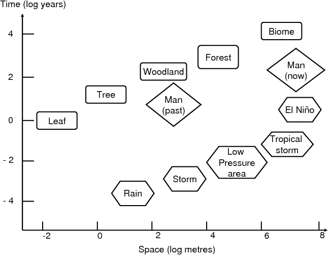
Fig. 1 shows a few spatio-temporal scales of living systems (here, forest) and of meteorological phenomena, while the two diamonds show the spatio-temporal influence range of pre-industrial and modern man, respectively. This kind of representation (without man) was introduced in 1986 by C.S. Holling¹. The figure illustrates how human influence on nature has changed: 10 000 years ago, there were 6 to 7 million humans. Nowadays, there are more than 6 billion – a thousand times more. 10 000 years ago, men were hunter-gatherers, and their action was at the scale of the leaf, or at most, at the scale of a tree. Nowadays, 300 km² of tropical forest are cut every day. Worse, the climate itself is impacted world-wide by human activity, leading in less than one century to changes that took thousands of years during past climatic variations. The biosphere was able to adapt to past changes because of genetic evolution, but now, the rate of change is too high to allow adaptive evolution or the migration of ecosystems along temperature or hygrometry gradients. Man-induced climate change also leads to the emergence of new diseases, or their extension to places where they were not present before, thus leading to major health concerns^{2, 3}.

To address those problems, scientists working in life sciences have to build models of the objects they study, and they have to follow the paths and methods which have previously been used by physicists to model and understand inanimate objects. As will be discussed later, mathematics is but a tool to achieve this goal.

This article does not intend to provide the reader with a complete understanding or an exhaustive inventory of existing modelling techniques for natural sciences, but simply to identify the goals and tools of modelling, and also its pitfalls. Above all, it attempts to convince the reader that work in collaboration with a physicist or a mathematician to build a model will offer rewards in the form of a better understanding. Modelling nature is not exclusive to the physicist or mathematician: it is the result of a team effort, where natural scientists are major players. Not only are they the end-users of an abstract product, but they are also essential in its making.

MODELLING: DEFINITION AND PRINCIPLES

The definitions of ‘model’ (noun) in the Compact Oxford English Dictionary are as follows:
(1) a three-dimensional representation of a person or thing, typically on a smaller scale
(2) a figure made in clay or wax which is then reproduced in a more durable material
(3) something used as an example
(4) a simplified mathematical description of a system or process, used to assist calculations and predictions
(5) an excellent example of a quality
(6) a person employed to display clothes by wearing them
(7) a person employed to pose for an artist
(8) a particular design or version of a product.
Obviously, what this article deals with is the definition provided in ‘4’, but ‘3’ is also relevant, as a given scientific model of a given phenomenon is sometimes an illustration of a larger class of phenomena (see for instance the ‘forest fire’ paradigm⁴). The automatic association of ‘mathematical’ with the activity of modelling in sciences is not a good one. In fact, mathematics (and therefore equations) is a tool used to build a scientific representation of reality. Modelling is based more on physics (as opposed to ‘metaphysics’) than on mathematics. The distinction is meaningful and will become obvious later in this article.

Science always follows a simple three-step process: (1) observation of a real phenomenon, e.g., the motion of planets, a tornado, the spread of a disease, the growth of a tree (2) elaboration of an abstract construction to represent or explain the observation; as seen earlier, it can be an equation, then called a law (like Newton’s law), a theory (which is basically a set of laws), or a model (3) comparison of the results or predictions of this construction with observation. If there is a strong disagreement, then go back to the second step.

Two points should be made here. First, the criterion of empirical falsifiability, introduced by Karl Popper, is essential to the scientific method in physics and many other sciences. A theory or a model cannot be ‘proven’ but only ‘refuted’ for logical inconsistency, or shown wrong by experimentation. A ‘good’ theory or model is one which withstands confrontations with experimentation. On the other hand, a conjecture in mathematics, which does not deal with physical objects, can be refuted (by a counter example) but can also be proven (and hence become a theorem). But a theory or a model can be wrong (as everybody knows, general relativity has replaced Newton’s theory of gravity), but can still be useful (planet orbits can be described with a good degree of accuracy using classical mechanics). Secondly, it is very important to make the distinction between prediction and understanding. A model can be purely descriptive. Models can have good predicting abilities, without incorporating underlying mechanisms – they are like a ‘black box’ into which one feeds input quantities, such as initial conditions, and which produce predicted quantities as output. Conversely, an explicative model is built from causal mechanisms and can therefore be termed a theory. Models which are oriented essentially towards prediction (often, statistical models) are different from those that are built mainly to help to understand a phenomenon (generally, mechanistic models). Nevertheless, once a good mechanistic model is built, it can also become useful for prediction.

Some other dichotomies should be defined, as listed below:

Static versus dynamic

A static model does not involve time, while a dynamic model does.

Spatial (usually 2-d or 3-d) versus local or non-spatial (0-d)

If the model is homogeneous (the system has the same state throughout), the variables are lumped, whereas if the model is heterogeneous (varying state within the system), then the variables are distributed or space-dependent.

Linear versus nonlinear

If all the equations in the model are linear equations, the model is known as a linear model. If one or more of the objective functions or constraints are represented by nonlinear equations, then the model is a nonlinear model.

Discrete versus continuous

In real life, one tends to consider that space, as well as time, are continuous. The phenomenon is then described by sets of either ordinary or partial differential equations (ODEs or PDEs). In many cases, however, models will consider space and/or time as discrete: time will proceed by jumps (which can be very short – fractions of seconds, or long – a year or more), while a surface will be described as a grid of squares and the variables will be computed on these squares. If the variables themselves are continuous, one speaks of finite difference equations (FDEs) (discrete time), or of coupled networks (discrete space and time). If the variables themselves take only discrete values, one will speak of cellular automata.

Deterministic versus probabilistic (stochastic)

A fully deterministic model performs exactly in the same way for a given set of initial conditions, while in a stochastic model, randomness is present and even when given an identical set of initial conditions, results may in some cases vary greatly (this would be the case for the outbreak of an epidemic started by one infected mosquito – if it dies before biting a host, there will be no incidence of the disease, whereas in another run of the model, the disease could reach the entire population). In other cases, the results have a limited dispersion, at least for averaged output variables (e.g., the epidemiological status of a given individual may vary from run to run, but the percentage of infected hosts would stay the same). The model is then said to be robust.

It is to be noted that mechanistic models can incorporate some randomness (for instance in the expression of transition rates between different states). They are then no longer fully deterministic, but if care is taken to verify the robustness, they can still be considered as explicative and mechanistic.

Top-down versus bottom-up

In many cases an idea or a theoretical model has been conceived before envisaging a specific application to a natural object. Reaction-diffusion equations and cellular automata were studied long before they were applied to morphogenesis of the patterns observed on shells and animal pelts (see, e.g., Ref. 5) or “tiger bush” in Niger⁶. This is also the case for collective behaviour theories, which were developed before their application to flocks of bird and schools of fish⁷. Such an approach can be classified as being “top-down” – from abstract concepts to practical application.

But often the problem comes first, and there exists no ready-made model or theory. The choice of modelling tools has to be decided after the question has been precisely formulated. It is then a “bottom-up” approach, from a practical problem towards an abstract formalization. Of course, once the modelling goal is reached, the physicist can try to find regularities and generalizations which can be compared to what is observed in more traditional physics.

MODELLING: TOOLS

A good modeller should be familiar with a number of concepts and methods. If one makes a short – and far from exhaustive – list, it should at least include the following: Hamiltonian theory, integrability, chaos, ergodicity, KAM tori, Lyapunov exponents, separatrices, jacobians, bifurcation theory, dissipative systems, (strange) attractors, fractals, percolation, solitons, deterministic models, stochastic models, probabilistic models, ODEs, PDEs, perturbation theory, FDEs, coupled lattices, cellular automata, wavelet analysis, neural networks, and Monte Carlo methods.

The reader should not be frightened by this list: it is only a toolbox. Modelling is the work of a team, and the most important thing is not the equations or the computer programs, but the exchange of information and ideas between the different specialists (ecologists, biologists, geologists, epidemiologists, etc. and physicists). It is only after constructive interactions between all of these specialists that the modeller (physicist or mathematician by training) can choose from their toolbox the relevant tools to make a model of the problem being addressed. The worst way to make a model is to work with somebody who is a specialist in one and only one of these mathematical tools, and who will not try to adapt their toolbox to the problem, but will bend reality to be compatible with the tool they know well. Again, a model is built at the crossroads of different scientific branches and the modeller is somebody who listens and catalyses the formation of ideas, relations, datasets and hypotheses, before writing equations. In addition, a scientific model is something that is never finished, as it has to be put into question again whenever new facts either contradict it or cannot readily be incorporated into it.

Many models have been proposed in recent years. They are often based on compartmental analyses and use a very wide range of methods from physics, mathematics, or statistics. It is important to know what one wants exactly before selecting which drawer of the toolbox to open first. Differential equations, coupled lattices, cellular automatons, stochastic processes, statistical estimations, non-parametric or semi-parametric methods, artificial neural networks analysis or sophisticated Markov chain Monte Carlo methods can be used in epidemiological or ecological modelling, but they will not all answer the same questions. There is no universal method to model complex systems in nature. The problem itself will lead to the choice of the method. For instance, multivariable statistical analysis is by itself a descriptive model from which one can infer underlying mechanisms and relations. Combined with multiple regression, it can be used to build predictive models which will be operational in the range of parameters covered by the data they use. But recent examples, such as the shameful dispersion in the predictions of BSE (bovine spongiform encephalopathy, or “mad cow disease”) epidemics of more than three orders of magnitude show the limits of such methods, which are ill adapted to extrapolate. Artificial neural networks can also be used for prediction⁸. Like traditional statistical methods, they rely on the integration of a large number of observations, but usually perform better. None of these methods gives an understanding of the object studied, but sometimes, for short-term prediction and optimization, they can be good choices: a good modeller will help the natural scientists to define their needs with precision and will identify the appropriate tools.

MODELLING: METHODS

From now on, we will talk only of explicative (mechanistic) models. To begin with, we can distinguish three steps in the mechanistic modelling of a natural system or process.

Ask the right question

In most cases, a global model of the object studied is not needed. Often, the question is down to earth, and the goals are urgent and practical: how to understand and protect a given type of ecosystem, how to save what can be saved, and otherwise, how to use its space and the life on it in an optimal way, and this at a given place and a given time. Confronted with such a well defined question which might seem simple but which in fact is often extremely complex, the physicist has to collaborate with the specialists of the other disciplines to determine what are the essential factors and variables, and what are the relations between them. In the case of the protection of a local ecosystem for instance, ecologists, botanists, and geologists will have to collaborate with economists, geographers, and sociologists, and the modelling processes starts with the confrontation of these different points of view. Only once a consensus has been reached on what are the essential ingredients can the choice of the mathematical tools be addressed. It is the same process in epidemiology: take the case of Rift Valley fever, first described in Eastern Africa in 1927 by Daubney et al⁹. The disease appeared in West Africa around 1989 and became endemic, although there was no wild animal reservoir for the virus. Epidemiologists¹⁰, entomologists¹¹, virologists¹², and other specialists took part in a joint effort which led to a mechanistic model¹³.

Choose the right tools

Mechanistic modelling has understanding as the primary goal. In French, “to understand” translates as “comprendre”, from the Latin cum-prehendere which means “to take together”. It is in essence a ‘complex systems’ approach, which puts together – as a mechanistic model – the hypotheses about the elementary processes. The mathematical tools are chosen from a large toolbox. Sometimes a suitable approach is not present, and new theoretical tools have to be developed specifically to address a new class of problems, e.g., small-world models¹⁴, variables aggregation^{15, 16}.

One could ask “what is best?” It is not a good question, because there is no unique answer. The method should be adapted to the problem being dealt with. To choose a method to model a real natural phenomenon, be it in ecology, biology, or epidemiology, the first thing is to properly define the real questions asked, and then to make an inventory of available data. If a modeller says they need several thousands of non-measurable parameters to build a model, they will get nowhere! Nevertheless, in some cases, additional data will have to be collected¹⁷, and in some others, it will even lead to the invention of new measuring methods e.g., see Ref. 18, or the discovery of unsuspected relations between measured parameters¹⁹. Secondly, one has to put together all the hypotheses on the possible mechanisms underlying the system. It is only then that one can choose a formal mathematical framework in which one will build the model. Once again, modelling nature is at the crossroads of many different scientific disciplines, and it is a team effort.

One should start with as minimal a model as possible (“small is beautiful”), and then develop it and compare its output with experimental data. The systematic exploration of the model parameter space will give an understanding of the behaviour of the system, and it will then be possible to compare its output with reality. It is only if the model is unsatisfactory that additional components should be added.

Analyse the results

Very often, the first model fails to reproduce the behaviour of the system studied. It is then necessary to reconsider the important factors, the mechanisms which link them, and to improve the model, which sometimes means that other factors and mechanisms have to be included. A good example is found in several problems in epidemiology, which cannot be modelled using a 0-d approach, and for which it has been shown that 2-d geometry has to be used (see, e.g., Refs. 13, 20). When a satisfactory agreement between observation and model output has been reached, it is then possible to make predictions and to study the effects of different strategies. Generally, one can observe the emergence of self-organization, which is a characteristic of complex systems and is the key to life, from the cell to the whole planet (Lovelock’s “Gaia” concept²¹). It is likely that it is because we subconsciously perceive this self-organization that we find some kind of beauty in most natural objects and landscapes. And if all living systems have a great ability to repair themselves and settle back to an equilibrium after a perturbation (this is called “resilience”), it is because of these self-organization properties. But there is always a limit beyond which repair is no longer possible, thus leading to the death of an organism, or – at a larger scale - to the disappearance of an ecosystem.

STARTING KIT: SUGGESTED READING

Scientists in the life sciences who are interested in modelling should try to interest physicists (or mathematicians with an open mind) in their problems. But before committing to a given scientist, they should be able to feel if the choice is good and therefore some personal investment on the basics would be helpful. Two good graduate level reminders of mathematics are the manuals by Mathews and Walker²², and by Arfken and Weber²³. A good general lecture on modelling methods was written recently by Boccara²⁴: it covers many of the tools mentioned above. An old classic on modelling in life sciences is that by D’Arcy Thomson²⁵; a recent study on the same topic was conducted by Murray⁵. Franc et al²⁶ provide a good review of modelling in forest ecology, while Anderson and May wrote a good book on epidemiology²⁷. Some classic papers in epidemiology modelling are those by Kermack²⁸, Anderson and May,^{29, 30}, and Hurd et al³¹. Ecological Modelling is an interesting journal which gives insights into the recent progress of modelling in various fields of life sciences and with many different techniques: see, e.g., papers on forest ecology by Chave³² and Moravie et al³³, and papers on epidemiology by Durand et al³⁴, Favier et al¹³, and Sabatier et al³⁵. The usefulness of satellite data can be seen for instance in Linthicum et al³⁶, Roberts et al³⁷, Thomson et al³⁸, and Thonnon et al¹⁰.

CONCLUSION: GOALS

To understand is a noble and important goal, but it is not the only one. Scientists have a responsibility to help decide the best policies. The most obvious goal is to keep the climate and the biosphere compatible with life, and to make sure the planet can feed people decently. But it is also important to maintain some protected areas, firstly to conserve biodiversity, but also for purely “aesthetic” reasons, to keep some “virgin” areas as witness of what the Earth was when man was less omnipresent. To achieve these goals, purely predictive tools based on previously accumulated data are likely to err badly when out of the range of their database. Mechanistic models are better candidates, as they allow a deep understanding of the complexity of a natural mechanism (e.g., of an ecosystem), including its self-organization properties and its resilience to perturbations. Modelling is not an expensive activity, but it brings very great rewards, and it should be actively pursued by scientists in every country.

Some inspirational reading is to be found in Arcadia by Tom Stoppard³⁹ from which the following extract is taken: “It makes me so happy. To be at the beginning again, knowing almost nothing. People were talking about the end of physics. Relativity and quantum mechanics looked as if they were going to clean out the whole problem between them. A theory of everything. But they only explained the very big and the very small. The universe, the elementary particles. The ordinary-sized stuff which is our lives, the things people write poetry about – clouds, daffodils, waterfalls – …these things are full of mystery, as mysterious to us as the heavens were to the Greeks.”

REFERENCES

1. Holling CS (1992) Cross-scale morphology, geometry, and dynamics of ecosystems. Ecol Monogr 62, 447–502.
2. Epstein PR (1999) Climate and health. Science 285, 347–8.
3. Rogers DL, Packer MJ (1993) Vector-borne diseases, models, and global change. Lancet 342, 1282–4.
4. Christensen K, Flyvbjerg H, Olami Z (1993) Self-organized critical forest-fire model: mean-field theory and simulation results in 1 to 6 dimensions. Phys Rev Lett 71, 2737–40.
5. Murray JD (1989) Mathematical Biology, Springer-Verlag, Berlin.
6. Thiery JM, Dherbes JM, Valentin C (1995) A model simulating the genesis of banded vegetation patterns in Niger. J Ecol 83, 497–507.
7. Grégoire G, Chaté H, Tu YH (2003) Moving and staying together without a leader. Physica D 181, 157–70.
8. Lek S, Guégan JF (2000) Artificial Neural Networks: Application to Ecology and Evolution, Springer-Verlag, Berlin.
9. Daubney R, Hudson JR, Garnham PC (1931) Enzootic hepatitis of Rift Valley fever, an undescribed virus disease of sheep, cattle and man from East Africa. J Pathol Bacteriol 34, 545–79.
10. Thonnon J, Picquet M, Thiongane Y, Lo MA, Sylla R, Vercruysse J (1999) Rift Valley fever surveillance in lower Senegal river basin: update 10 years after the epidemic. Trop Med Int Health 4, 580–5.
11. Fontenille D, Traore-Lamizana M, Diallo M, Thonnon J, Digoutte JP, Zeller HG (1998) New vectors of Rift Valley fever in West Africa. Emerg Infect Dis 4, 289–93.
12. Zeller HG, Fontenille D, Traoré-Lamizana M, Thiongane Y, Digoutte JP (1997) Enzootic activity of Rift Valley fever virus in Senegal. Am J Trop Med Hyg 56, 265–72.
13. Favier C, Chalvet-Monfray K, Sabatier P Lancelot R, Fontenille D, Dubois MA (2006) Rift Valley fever in West Africa: the role of space in endemicity. Trop Med Int Health 11, 1878–88.
14. Kuperman M, Abramson G (2001) Small world effect in an epidemiological model. Phys Rev Lett 86, 2909–12.
15. Auger P, Bravo de la Parra R (2000) Methods of aggregation of variables in population dynamics. Compt Rendus Acad Sci III 323, 665–74.
16. Pongsumpun P, Garcia Lopez D, Favier C, Torres L, Llosa J, Dubois MA (2008) Dynamics of dengue epidemics in urban contexts. Trop Med Int Health 13, 1180–7.
17. Charles-Dominique P, Chave J, Dubois MA, De Granville J-J, Riera B, Vezzoli C (2003) Colonization front of the understorey palm Astrocaryum sciophilum in a pristine rain forest of French Guiana. Global Ecol Biogeogr 12, 237–48.
18. Cournac L, Dubois MA, Chave J, Riéra B (2000) Fast determination of light availability and leaf area index in tropical forests. J Trop Ecol 18, 295–302.
19. Dubois MA, Sabatier P, Durand B Calavas D, Ducrot C, Chalvet-Monfray K (2002) Multiplicative genetic effects in scrapie disease susceptibility. Compt Rendus Biol 325, 565–70.
20. Favier C, Schmit D, Müller-Graf CDM, Cazelles B, Degallier N, Mondet B, Dubois MA (2005) Influence of spatial heterogeneity on an emerging infectious disease: the case of dengue epidemics. Proc Roy Soc Lond B 272, 1171–7.
21. Lovelock JE (1979) Gaia: A New Look at Life on Earth, Oxford Univ Press, Oxford.
22. Mathews J, Walker RL (1970) Mathematical Methods of Physics, Addison.
23. Arfken GB, Weber H (2001) Mathematical Methods for Physicists, Academic Press.
24. Boccara N (2004) Modelling Complex Systems, Springer-Verlag, Berlin.
25. D’Arcy Thompson (1917) On Growth and Form, reissued in 1942 by Cambridge Univ Press.
26. Franc A, Gourlet-Fleury S, Picard N (2000) Une introduction à la modélisation des forêts hétérogènes, ENGREF, Nancy.
27. Anderson RM, May RM (1991) Infectious Diseases of Humans: Dynamics and Control, Oxford Univ Press, Oxford.
28. Kermack WO, McKendrick AG (1927) A contribution to the mathematical theory of epidemics. Proc Roy Soc Lond A 115, 700–21.
29. Anderson RM, May RM (1979) Population biology of infectious diseases, Part I. Nature 280, 361–7.
30. May RM, Anderson RM (1979) Population biology of infectious diseases, Part II. Nature 280, 455–61.
31. Hurd HS, Kaneene JB (1993) The application of simulation models and systems analysis in epidemiology: a review. Prev Vet Med 15, 81–99.
32. Chave J (1999) Study of structural, successional and spatial patterns in tropical rain forests using TROLL, a spatially explicit forest model. Ecol Model 124, 233–54.
33. Moravie M-A, Pascal J-P, Auger P (1997) Investigating canopy regeneration processes through individual-based spatial models: application to a tropical rain forest. Ecol Model 104, 241–60.
34. Durand B, Dubois MA, Sabatier P, Calavas D, Ducrot C, Van de Wielle A (2004) Multiscale modelling of scrapie epidemiology. II. Geographical level: hierarchical transfer of the herd model to the regional disease spread. Ecol Model 179, 515–31.
35. Sabatier P, Durand B, Dubois MA, Ducrot C, Calavas D, Van de Wielle A (2004) Multiscale modelling of scrapie epidemiology. I. Herd level: a discrete model of disease transmission in a sheep flock. Ecol Model 180, 233–52.
36. Linthicum KJ, Anyamba A, Tucker CJ, Kelley PW, Myers MF, Peters CJ (1999) Climate and satellite indicators to forecast Rift Valley fever epidemics in Kenya. Science 285, 397–400.
37. Roberts DR, Paris JF, Manguin S, Harbach RE, Woodruff R, Rejmankova E, Polanco J, Wullschleger B, Legters LJ (1996) Prediction of malaria vector distribution in Belize based on multispectral satellite data. Am J Trop Med Hyg 54, 304–8.
38. Thomson MC, Connor SJ, Milligan P, Flasse SP (1997) Mapping malaria risk in Africa: What can satellite data contribute? Parasitol Today 13, 313–8.
39. Stoppard T (1993) Arcadia, Faber & Faber.